Everyone has seen a topographical map at some point during their life. In addition to the information that regular maps have, topographical maps typically show land features and elevation. How are these maps generated? Given that it’s not possible to sample the elevation at every single point in the area of interest, we must use some sort of interpolation. To tackle this mathematically, we should make a few simplifications.
As you might agree, the Earth is round. However, if we consider the Earth to be a differentiable closed manifold, it is locally linear. That is, in a reasonably small region, the surface of the Earth can be approximated with a flat plane. That allows us to model the elevation in this region as a scalar function of two position variables. Each point in the region is associated with its elevation. Since we can’t measure an infinite number of points in this region (try it if you don’t believe me), we are forced to settle for a finite sample. But we still want accurate elevation numbers for the areas we don’t measure directly. To make the problem more concrete, suppose we have elevation measurements at the black points and we want to find a good approximation for the elevation at the red point:
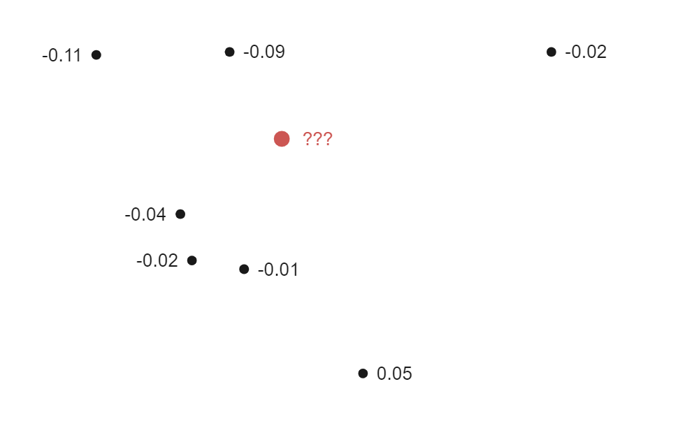
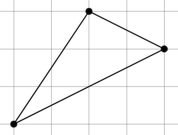
We can do this by interpolating between the values that we do have access to. There are many ways to go about it, such as a $k$-nearest neighbors approach, but this article will focus on using Delaunay Triangulation, a method from a branch of math known as computational geometry. To determine the elevation of the red point, we only want to consider points that are immediately around it. The height at the points that are further away likely don’t tell us as much about the height at the red point. We can use a point-set triangulation for this. If you look up “point-set triangulation” on the internet, you’ll see some mystic nonsense about “simplicial complexes” and a bunch of other fancy words that some stuffy guy probably made up a hundred years ago. Don’t worry, because you don’t need to know any of that terminology to understand triangulation, which is a pretty simple concept. Triangulation is the process of generating a mesh of triangles that cover the convex hull of a set of points. The triangles shouldn’t overlap and every triangles’ vertices should be in the set of points. This is easier to understand with pictures. If you have this set of points:

This is a potential triangulation:

As mentioned before, we don’t want to give much weight to points that are far away from a given point of interest. For this reason, sliver triangles, or triangles with small minimum interior angles, are bad for interpolation. Consider this example with elevation measurements at four points:
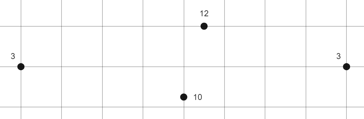
Just by inspection, the data suggests that there is a ridge or hill along the line of the two middle points. Now suppose we want to use a triangulation to approximate the elevation at the red point, which is probably part of the same hill:

There are two possible triangulations for this set of black points. Let’s call them triangulation 1 and triangulation 2 for reference.

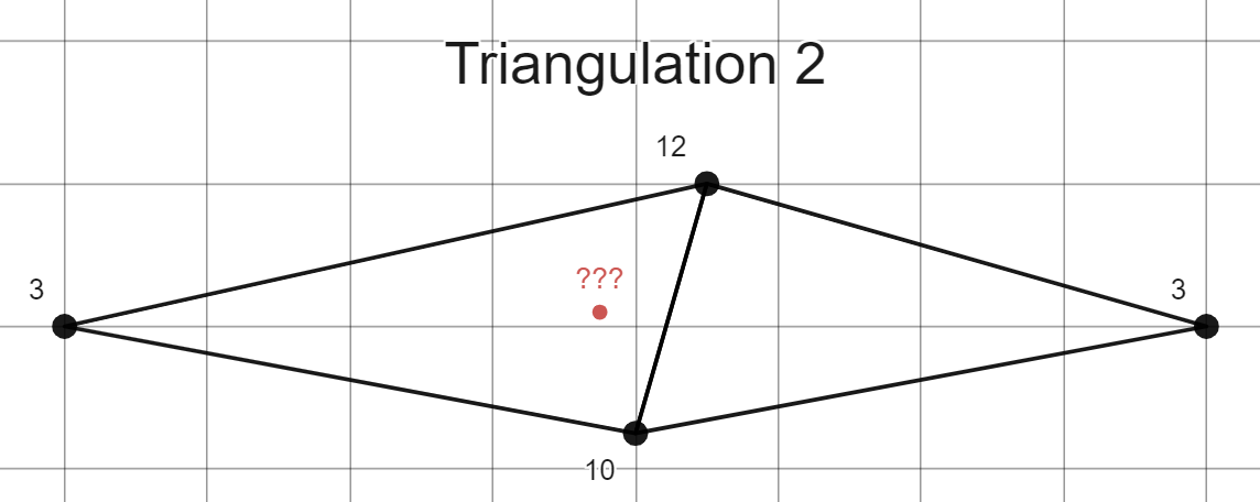
Triangulation 1 has sliver triangles. Using triangulation 1, the two strongest influencers on the estimated value of the red point are the points far away to the left and right. This would result in a low elevation estimation for the red point, contradicting the earlier observation that the red point is likely part of a hill along the two center points. The triangles in triangulation 2, on the other hand, have larger minimum angles. Using this, the middle points have the strongest influence on the estimation for the red point. This results in a higher value, which conforms better to our expectations.
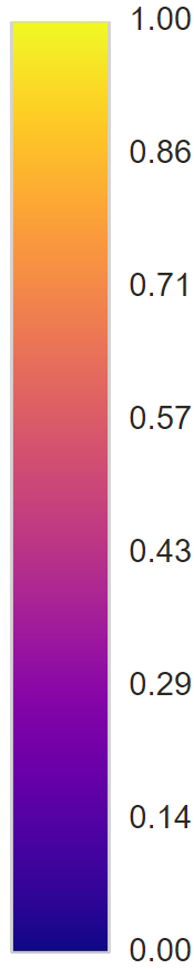
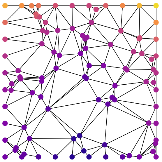
We can use this idea to measure how good a given triangulation is by calculating and listing the minimum interior angles of each triangle. This is where the Delaunay triangulation comes in. The Delaunay triangulation maximizes the minimum interior angle, reducing sliver triangles. A Delaunay triangulation is any triangulation that satisfies the “Delaunay condition”: no point in the set is contained within the circumcircle of any of the triangles. This triangulation is unique in most cases, and exists for all sets of points that are not all collinear. Now, at any given point, we can linearly interpolate between the height values at the vertices of the Delaunay triangle that contains it. Suppose we have this set of points in the plane, where color represents elevation according to the following scale:
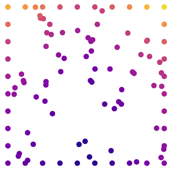
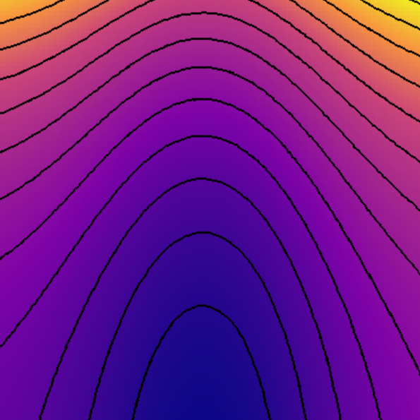
Applying the Delaunay triangulation and linearly interpolating as described above, we can get a smooth heightmap:

Once we have these interpolated values, we can use an isoline generating algorithm to produce contour lines if desired. To generate this image, I used marching squares (see reference [5]):
Constructing the Delaunay triangulation can be done in a variety of ways, but here we will discuss the most intuitive method, known as the flip method. Note that the flip method has $O(n^2)$ worst-case runtime, and that more optimized methods exist. For further reading on Delaunay construction, see references [1], [2], and [3] at the bottom of the post. For a series of videos that cover the Delaunay triangulation in a more technical manner, see reference [4].
As mentioned before, we must satisfy the Delaunay condition. We can guarantee this by generating an arbitrary triangulation and fixing triangles that don’t meet the condition, using a “flip” operation. Suppose these are the first three points of a point set we want to triangulate:
We proceed by adding the next point and connecting it such that edges do not overlap. I’ve added some labels to the diagram for easier reference.
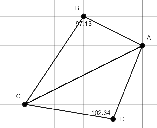
Here, ∠$B + $∠$D \geq 180°$. For the Delaunay condition to be satisfied, the angles across from the connecting edge must sum to an angle less than $180°$ (The proof of this equivalence is beyond the scope of this post, but can be found in reference [4]). Note how the circumcircles contain points in the point set:

So we perform a flip operation: we remove the problematic edge and replace it with one going the other way:
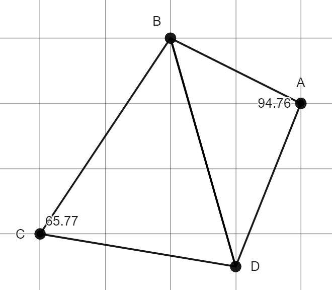
Here, ∠$A +$∠$C \lt 180°$, so the Delaunay condition is satisfied. To check, here are the circumcircles of each triangle.
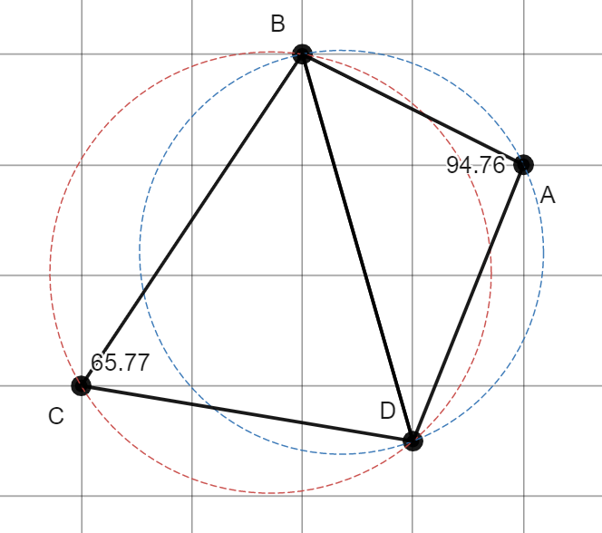
Note how the circumcircles no longer contain any points in the point set: the Delaunay condition is satisfied. The flip operation is mathematically guaranteed to increase the maximum minimum angle of the triangles. The proof of this fact is in reference [4]. To complete the triangulation, we continue adding points one by one and flipping edges to ensure it satisfies the Delaunay condition.
Thanks for reading! Hope you got something out of it.
(Disclaimer: I don’t really think the people who created and studied Delaunay triangulations are “stuffy guys from a hundred years ago” – I’m just messing around and I have a lot of respect for the work of those people. The jargon is useful, it’s just unnecessary and distracting for the concepts at the level I’ve presented them here.)
This post was submitted to the SoME2 contest.
All images created with Desmos (reference [6] and [7]) or MathGraph3D.
References
[1] http://www.personal.psu.edu/cxc11/AERSP560/DELAUNEY/13_Two_algorithms_Delauney.pdf
[2] https://en.wikipedia.org/wiki/Delaunay_triangulation
[3] https://en.wikipedia.org/wiki/Bowyer%E2%80%93Watson_algorithm
[4] https://youtube.com/playlist?list=PLubYOWSl9mIuEaEho05RoZy9OKpNE843H
[5] https://en.wikipedia.org/wiki/Marching_squares
[6] https://www.desmos.com/calculator/p5o7l7xqcg
[7] https://www.desmos.com/calculator/imicofl2p6
[8] Not exactly a reference but bn̈ue̤ ɯ́mem̑ə̮ from a discord server I’m in noticed a certain pattern in the points from my sample images: https://imgur.com/0NoU8Jb