This series focuses on the creation of the original version of my 3D plotting software MathGraph3D. This first part is concerned with the overall structural components of the software.

Before getting into any actual algorithms or math, it’s necessary to set up an outline for how the code will be structured. I decided to create a manager class called “Plot” that would handle everything to do with 3D space and all objects in the calculator. There are five main operations that the Plot must be able to do (among other smaller operations):

• Determine the bounds and scale of the 3D space. The user should be able to input upper and lower bounds for each axis, and this defines the space used by the calculator.
• Projects points in 3D to cartesian points in 2D, then finally to canvas coordinates, relative to the top left of the screen, to be drawn. Typically, this is done with a camera and matrices for rotation and projection. But the original version of MathGraph did not use this because I wasn’t familiar with matrix math, so I developed my own algorithm for projection. However, both will be covered in this series for the sake of its usefulness.
• Occlusion of shapes. I decided to go with the Painter’s method for occlusion. Since MathGraph3D does not operate with pixel-perfect access, better algorithms are mostly out of reach. “Occlusion” means that when an object (polygons and lines) is obscured or blocked by another object from the perspective of the view, it is not drawn to the screen. However, the Painter’s method is imperfect and sometimes results in ambiguous situations. Take, for example, the scenario in which two polygons intersect at a line through their centers. There is no way to decide which polygon should be in front because both are partially obscured by the other. To handle this, I developed a modification on the standard algorithm that will be discussed later.
• Drawing Everything to the Canvas. This includes functions, points, vectors, geometry, the axes, axis numbers, etc.
• Clipping. Objects on the Plot should never exceed the bounds of the defined 3D space. For example, assume all axes range from -4 to 4. The function $f(x,y)=x^2+y^2$ will exceed the upper z bound at input values outside the circle centered at the origin with radius 2. But I don’t want the part of the surface that goes outside the bounds to be shown; it should be “clipped” at the boundary. The same goes for all bounding planes (x=-4, x=4, y=-4, y=4, z=-4, z=4) and any additional ones defined by the user.

The next step for baseline setup is the general “Plot object” class, from which every surface should inherit. This will be covered in the next post. The final main structural component of the code is the GUI, but that is not discussed here. Now, we can get into the details of the Plot object. I’ll discuss the main operations of the PLot in the order they are outlined above.

Determining the bounds and scale of the 3D space

This operation involves determining the position of the axes and the origin based on bounds, the scale per unit in each direction based on the axis length, and the number of units in each direction.

It is easy to find the number of units; it’s just the length of the interval between the upper and lower boundaries. To compute that, you can subtract the lower boundary from the upper one. To find the unit scales, you can take the axis length and divide it by the number of units along that axis. For example, if one of the axis lengths is 500 pixels and the user wants it to range from -5 to 5, there are 5 – (-5) = 10 units, so there are 500 pixels / 10 units = 50 pixels per unit.

The problem is actually a bit more complicated than that because all axes are not necessarily the same length but they should be the correct length relative to each other. In other words, if one axis has 10 units and another has 5, the first should appear twice as large as the first. Solving this will automatically yield the correct position of the origin.

3D Projection – version implemented in the original MathGraph3D

I’ve written about my algorithm before, and it’s buried deep somewhere on this website as a PDF. It’s not very high quality, so I’ll take this opportunity to rewrite it more clearly.

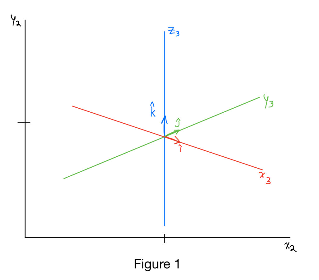
Figure 1 shows the three dimensional axes $x_3$, $y_3$, and $z_3$. These are the axes for the three dimensional points to be projected. $\hat{i}, \hat{j}, \hat{k}$ are the units of the $x_3$, $y_3$, and $z_3$ directions, respectively. $x_2$ and $y_2$ are the two-dimensional axes onto which the 3D points are to be projected.

Since any point can be expressed as a linear combination (scaled sum) of the unit vectors, the problem of projecting any 3D point to 2D is a matter of finding the projected unit vectors.Then any 3D point $\left(a, b, c\right)$ may be projected like this, where $\text{P}=\left(x_p, y_p\right)$ is the result: 

$$x_p=a\cdot \hat{i}_x + b \cdot \hat{j}_x + c\cdot \hat{k}_x \\y_p=a\cdot\hat{i}_y + b\cdot\hat{j}_y + c\cdot\hat{k}_y$$

Written in matrix form,

$$\text{P}=\begin{bmatrix}a&b&c\end{bmatrix}\begin{bmatrix} \hat{i}_x & \hat{i}_y \\ \hat{j}_x & \hat{j}_y \\ \hat{k}_x & \hat{k}_y \end{bmatrix}=\begin{bmatrix}a\hat{i}_x+b\hat{j}_x, a\hat{i}_y+b\hat{j}_y+c\hat{k}_y\end{bmatrix}$$

It’s worth noting that in the original version’s code, the multiplication of $c$ and $\hat{k}_x$ is not actually computed because the z axis is fixed to always be straight up and down. This means $\hat{k}_x$ is always going to be zero so doing this computation is a waste.

Let $y’$ be the line normal to the plane formed by $x_2$ and $y_2$ and let $\alpha$ be the angle between $x_2$ and $y_2$ in the plane formed by $x_2$ and $y’$. Then $\alpha$ corresponds to rotation about the z axis in 3D space. Let $\beta$ be the angle formed between $y_2$ and $z_3$ in the plane formed by $y_2$ and $y’$. So $\beta$ corresponds to rotation about a stationary horizontal axis in the 3D space.

$\hat{k}$ is the easiest unit vector to find because its projected x value never changes.

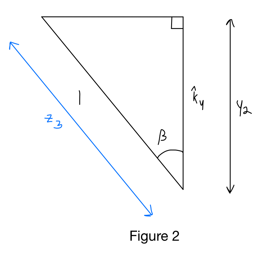
In Figure 2 it can be seen that:

$$\hat{k}_y = \cos\left(\beta \right) \implies \hat{k}_{\text{projected}} = \left(0, \cos\left(\beta \right) \right)$$

Finding the projected x of $\hat{i}$ is straightforward, but the projected y is a bit more difficult.

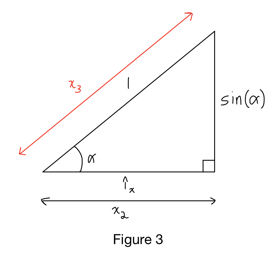
Figure 3 shows that $\hat{i}_x=\cos\left(\alpha \right)$. If we take the side of the triangle with $\sin\left(\alpha \right)$ and project it onto the plane formed by $y_2$ and $y’$ and angle $\beta$, this triangle is obtained:

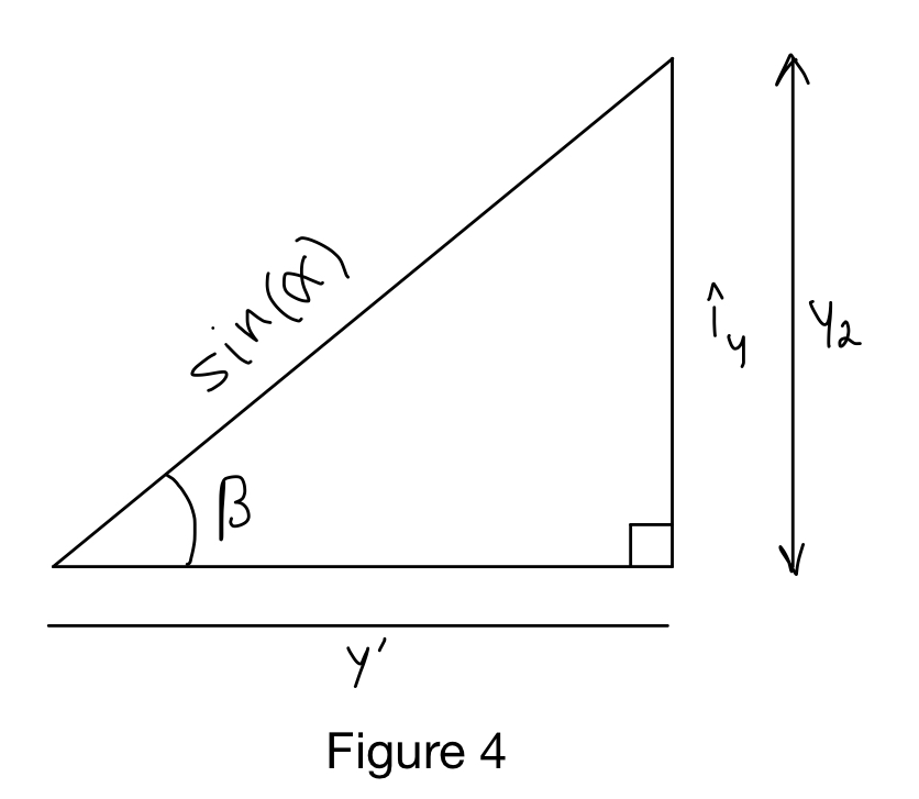
Figure 4 shows:

$$\sin\left(\beta \right) = \frac{\hat{i}_y}{\sin\left(\alpha \right)} \implies \hat{i}_y = \sin\left(\alpha \right)\sin\left(\beta \right)$$

$$\text{So } \hat{i}_{\text{projected}} = \left(\cos\left(\alpha \right),\sin\left(\alpha \right)\sin\left(\beta \right)\right)$$

The angle in the same plane as $\alpha$ but between $x_2$ and $y_3$ is $\alpha+\frac{\pi}{2}$ because $x_3$ and $y_3$ are perpendicular. Therefore $\hat{j}_x$ must be

$$\cos\left(\alpha + \frac{\pi}{2}\right) = -\sin\left(\alpha \right)$$

Since $\sin\left(x+\frac{\pi}{2}\right)=\cos\left(x\right)$. So the same triangle as in figure 4 can be used except with $\cos\left(\alpha \right)$ instead of $\sin\left(\alpha \right)$ and $\hat{j}_y$ instead of $\hat{i}_y$:

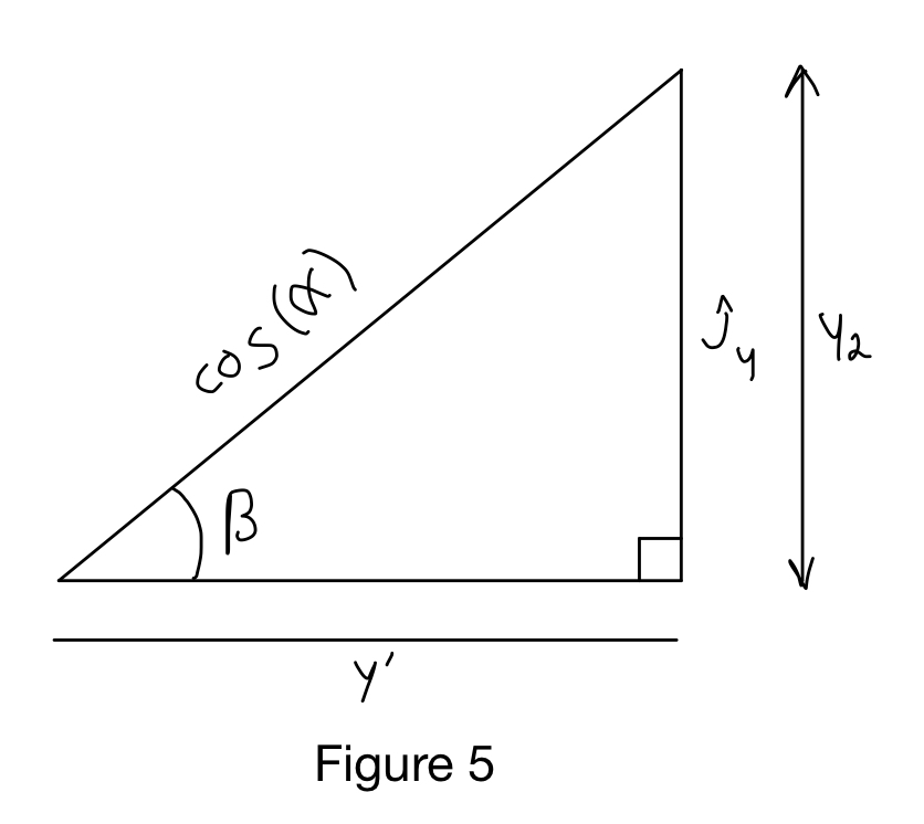
We can see from Figure 5 that:

$$\sin\left(\beta \right) = \frac{\hat{j}_y}{\cos\left(\alpha \right)} \implies \hat{j}_y = \cos\left(\alpha \right)\sin\left(\beta \right)$$

$$\text{So } \hat{j}_{\text{projected}} = \left(-\sin\left(\alpha \right), \cos\left(\alpha \right)\sin\left(\beta \right) \right)$$

Summarizing,

$$\hat{i}_{\text{projected}} = \left(\cos\left(\alpha \right),\sin\left(\alpha \right)\sin\left(\beta \right)\right)$$

$$\hat{j}_{\text{projected}} = \left(-\sin\left(\alpha \right), \cos\left(\alpha \right)\sin\left(\beta \right) \right)$$

$$\hat{k}_{\text{projected}} = \left(0, \cos\left(\beta \right) \right)$$

Occlusion of shapes

In order to implement the Painter’s method, we must have a way to determine which shapes are closest to the view at any angle. Initially, I went case by case and determined the closest octant to the viewer and sorted the polygons according to its outer corner. This, however, is imperfect. So once again I began to create my own algorithm. I’m somewhat of a chaotic worker with most of my progress and ideas coming in bursts, which means when inspiration strikes I have to find the quickest way to get the idea out on paper before I forget it. Unfortunately, I can’t find the scrap of paper where I originally derived my algorithm for this, and at the moment I can’t rederive it, so I’ll present the formula here and hopefully update this post if I find the paper or remember my train of thought.

The idea behind this algorithm is to find the point of intersection between a ray originating at the viewer’s eye and a sphere centered at the origin with given radius $r$. The polygons can then be sorted in reverse by squared distance from the intersection point and they will be drawn in the correct order, accounting for occlusion. For efficiency reasons, squared distance is used instead of actual distance, as the square root calculation is computationally expensive. The squared distance will preserve the correct order, as $\sqrt{x}$ is injective and monotonically increasing across the positive numbers. Anyway, suppose the intersection point is called $Q$. Let $\theta = -\left(\alpha +\frac{\pi}{2}\right)$ and $r$ be the radius of the sphere centered at the origin. Then the coordinates of $Q$ are given by:

$$Q = \left( r\cos\left(\theta \right), r\sin\left(\theta \right), \left| r \right| \sin\left(\pi – \beta \right) \right)$$

I’m not sure what the absolute value signs are there for, because this formula works fine for any positive radius. It’s probably there in case I wanted to have a negative radius for some reason, but it’s perfectly acceptable to leave it out.

The modification on the Painter’s algorithm that I referred to earlier is splitting polygons to handle overlap. This modification was not included in the first version, but it’s worth including here. It works by checking every single polygon against every other one, and if there’s overlap, splitting both polygons into two pieces at the line of intersection. Solving for the line of intersection between two planes in space is a basic linear algebra problem, and there are many resources online that show how to compute it so I won’t cover it here. The only difference is that the polygons are plane regions, not entire planes. But resolving this difference is only a matter of restricting the boundaries of the plane on which the polygon lies.

Surface Clipping

The original version of MathGraph3D only allowed clipping for planes equal to z=c for some constant c. I’ll cover the general plane clipping method in this post anyway. We want an algorithm that can take in the normal vector of a plane and a point that lies on the plane, and replace all points on the side to which the normal points (the “outside”) with interpolated points on the plane itself. This is done by first identifying which points are on the outside, then computing the intersection of the segment formed between each outside point and the nearest inside point of a polygon. If all points are outside, the polygon is removed entirely; if no points are outside, the polygon is kept as is. Call the normal vector $\vec{n}$ and the point lying on the plane $\vec{R}$. Then, the clipping plane precomputes the test value $T = \vec{n} \cdot \vec{R}$. All points on the outside of the plane, when dotted with the normal vector, will produce a value greater than $T$. Therefore, the following test can be used for a point $\vec{S}$:

$$\vec{n}\cdot \vec{S} – T > 0$$

If the test is true, $S$ is outside the clipping plane. Otherwise, it is on the inside. Now, given an outside point $P_{\text{out}}$ and an inside point $P_{\text{in}}$, we need to find the point on the clipping plane that lies between them. First, the direction vector of the line between these points is computed: $\vec{d} = P_{\text{out}} – P_{\text{in}}$. We then compute the value of the parameter $t$ at which the line between these two points intersects the clipping plane: 

$$t=\dfrac{\vec{n} \cdot (\vec{R} – P_{\text{out}})}{\vec{n}\cdot \vec{d}}$$

From here, computation of the intersection point is easy:

$$ P_{\text{out}} + t\cdot \vec{d} $$

Each new polygon is made up of the inside points and the computed boundary points, all sorted clockwise.