Due to the COVID pandemic, the Susceptible-Infectious-Removed (SIR) model for disease spread has grown wildly in popularity. SIR is a system of differential equations that models the evolution of a disease over time. Knowledge of the SIR model is not necessary to understand this post, but there are many great videos about it online if you want to learn more. My favorites are: Simulating an epidemic by Grant Sanderson, Oxford Mathematician explains SIR Disease Model for COVID-19 (Coronavirus) by Dr. Tom Crawford, and The Coronavirus Curve – Numberphile by Ben Sparks.
Differential equation modelling is not limited to disease spread. As a student of French, I wanted to apply it to language learning progression. It actually wasn’t that hard to nail down a pretty convincing representation. In this post, I’ll outline the model, explain how to obtain numerical solutions, how the model could be improved, and of course, turn the data into a 2D surface (embedded in three dimensions).
The basic premise is to assume that when learning, knowledge of all aspects of the language (grammar, vocabulary, pronunciation, listening comprehension, and so on) fall into three categories: “Unknown”, “Familiar”, and “Mastered”. “Unknown” (U) refers to aspects of language that have not yet been encountered or that have been practically forgotten. “Familiar” (F) refers to aspects of language that are known, but are not mastered. “Mastered” (M) refers to what has been learned completely and is available in a person’s working memory. The model will be called the Unknown-Familiar-Mastered (UFM) model from now on.
$U$, $F$, and $M$ must always sum to exactly one because they represent the proportion of the language that is in their respective categories. $dU/dt$, $dF/dt$, and $dM/dt$ are all functions of the four variables $t, U, F,$ and $M$ because the rate of change of each variable depends on time (t) and the current value of each variable. They also rely on the constant parameters $\alpha$ and $\beta$ that range from 0 to 1. The parameter $\alpha$ measures how quickly the individual in question learns new information. The parameter $\beta$ measures how quickly the person forgets or loses proficiency in information they have already learned. Assuming zero prior knowledge of the language, the initial conditions at $t=0$ are $U(0)=1$, $F(0)=0$, and $M(0)=0$. In other words, all is unknown, and nothing is familiar or mastered. All that is left to cover is how to write expressions for the rates of change of each variable.
First, consider $dU/dt$. It is equivalent to the rate of change of how much of the language is completely unknown or forgotten. What causes the unknown amount to change? There are two things: learning new information, and forgetting information that is familiar. It is unlikely that information would go directly from being mastered to completely unknown, so this does not need to be taken into account. To represent learning new information, we can add the term $-\alpha U$. By multiplying the learning rate $\alpha$ and the unknown amount $U$, we get the amount of unknown material learned per unit time. When something is learned, it is removed from the unknown category, thus the negative sign. To account for forgetting familiar stuff, we can use the term $\beta F / (2\alpha+ 1)$. $\beta F$, the rate of forgetting times the familar amount, gives the amount forgotten from the familar category per unit time. Since $\alpha$ is always at most zero, the denominator of this term is always at least 1, so the amount forgotten will never exceed $\beta F$. $\alpha$ is in the denominator because a better learner is less prone to losing knowledge. This leaves:
$$\frac{dU}{dt} = -\alpha U + \frac{\beta F}{2\alpha + 1}$$
as the first of the three derivatives in the system. Next, skip over familiar and consider $dM/dt$. Again, we must consider what causes the amount mastered to change. Like before, it depends on how much is learned and how much is forgotten. Since nothing can immediately go from unknown to mastered, the only growth or loss will be due to exchanges with the familiar category. Assuming a person is less likely to forget things that are mastered, we can make the forgetting term equal to half of what is was in the unknown category and replace $F$ with $M$: $-\beta M / (4\alpha +2)$. This time, it is negative because forgetting in this case removes knowledge from the category. To account for learning, we add a similar term to before, $\alpha F$. This is equivalent to the amount mastered from the familiar category per unit time. This leaves:
$$\frac{dM}{dt} = -\frac{\beta M}{4\alpha + 2}+\alpha F$$
The last category, Familiar, is easy because it’s the sum of these previous two derivatives with the signs flipped. Both Unknown and Mastered are only allowed to exchange with Familiar, so the rate of change of Familiar is the opposite of the sums of the changes in the other categories, leaving:
$$\frac{dF}{dt} = -\frac{\beta F}{2\alpha + 1} – \alpha F + \frac{\beta M}{4\alpha + 2} + \alpha U$$
Obviously, these expressions could be algebraically simplified. However, I find that doing so obscures the intuitive meaning of each term, so they are better off the way they are.
Now, how can we use these equations to get the actual values of $U, F,$ and $M$? As with Pursuit Curves, we can use the numerical 4th order Runge-Kutta method. Pursuit curves only required finding the solution to a single differential equation, but this application requires finding the solution to a system. This makes things slightly different, but it is actually quite similar because using a vectorized form, it is possible to write the entire system as a single equation. By letting $y=(U,F,M)$, we can write:
$$\frac{dy}{dt}=f(t,y)$$
where $f_i$ is the expression for the derivative of $y_i$ with respect to $t$. The initial conditions mentioned above can be written as $y(0)=y_0$ where $y_0=(U(0),F(0),M(0))$. Given these forms, we can apply the Runge-Kutta method as usual.
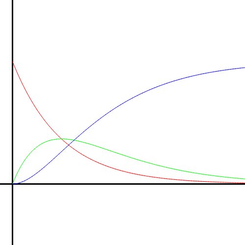
Using this numerical method, I created graphs of the solutions to the UFM system. Here is how the solution curves look as $\alpha$ and $\beta$ change. Red is Unknown, green is Familiar, and blue is Mastered.

Notice how the unknown curve slopes downward until it is near zero, and the mastered curve slopes quickly up towards 1. This corresponds to the ideal situation, where the language is learned as fast as possible because the person is a quick learner who never forgets anything.
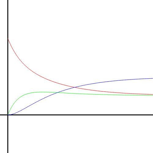
When $\alpha$ is lowered to half, the solution curves are the same shape but spread across a longer period of time because the person does not learn as quickly.

The same thing happens here. This $\alpha$ value corresponds to a very slow learner (who still doesn’t forget anything). The curves are very stretched out at this point, meaning it would take forever to learn the whole language. If $\alpha$ was lowered all the way down to zero, all the lines would be perfectly horizontal, never changing from their initial conditions. In other words, no progress would be made at all.
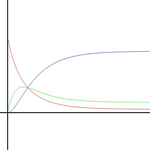
Bringing $\alpha$ back up to the max, this clearly corresponds to someone who learns quickly. However, as $\beta$ is also 1, the person never actually reaches 100% mastery. They forget things at such a rate that it causes them to plateau.
Lowering $\alpha$ while keeping $\beta=1$ makes the plateau’s maximum height decrease, i.e. the person does not learn as much before their forgetting catches up to them.
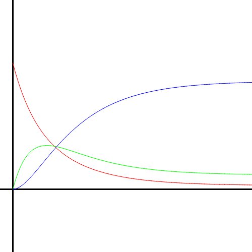
This is what I call the “realistic” case. $\beta$ is high enough to stunt the learning but not quite high enough to cause a complete plateau. $\alpha$ is big enough to attain a good height before the effects of $\beta$ really start to take hold. This is realistic because learning usually happens faster than forgetting (with regular practice) and it’s not reasonably possible to attain 100% proficiency.
(If you want to mess around with $\alpha$ and $\beta$ yourself, I created this Geogebra graph with the equations: https://www.geogebra.org/calculator/zvqbetv7. All images in this post were generated with my own software, not Geogebra.)
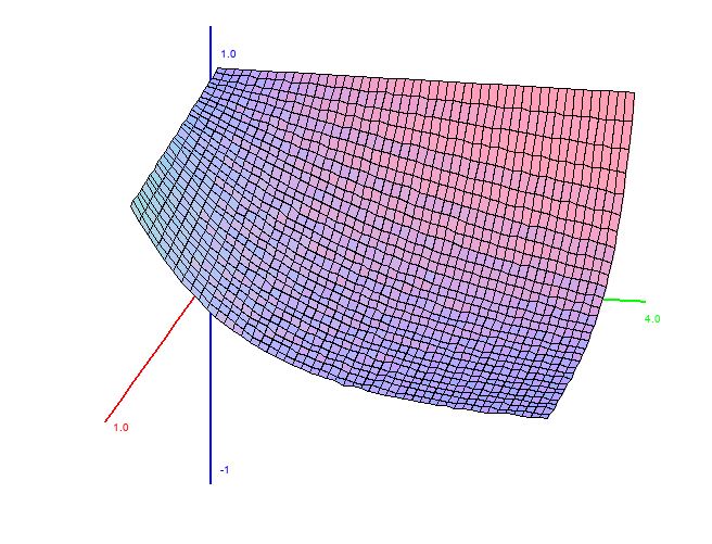
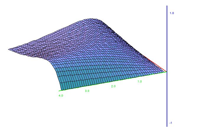
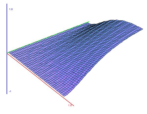
Now, as promised, here come the surfaces. By fixing $\beta$ and letting $\alpha$ vary, we get a sequence of curves. If we plot $\alpha$ on the $x$ axis and the curves along the $y$ and $z$ axes, we end up with a surface. This also works if you let $\beta$ vary while $\alpha$ is fixed. Using MathGraph3D python version StatisticalPlots.StatPlot3D, that’s exactly what I did. This post only includes the $\alpha$-variant surfaces because the $\beta$-variant surfaces are not different enough along the $\beta$ axis to look good. The red axis is the $\alpha$ axis.

Obviously, just like the SIR model, the UFM model makes a lot of assumptions and simplifications. This is a necessity – it would not be possible to model everything, so we need to make simplifications in order to make things mathematically feasible. However, that is not to say this model cannot be improved. Here, we’ve assumed that $\alpha$ and $\beta$ are constant over time (and furthermore, that all learning and retention ability can be encapsulated with two parameters). This is likely untrue. We probably forget less when we’re more familiar with the language, and learn faster when we already have some knowledge. If you’re unconvinced, consider that I’m only speaking from personal experience with my years of learning French. Still, we probably learn faster when we have more knowledge because much of language learning is done through inference in context. The more you know, the more context it is possible to understand, so the easier it is to infer.
I hope you enjoyed this post. If you did, please share it. Thanks for reading!