“Mathematical beauty” usually refers to the elegance of a proof, that is, how cleanly some mathematical result is proven with a convincing argument. That certainly sounds appealing to those who are already immersed in math, but it’s not clear how such a result is “beautiful” in the general sense of the word. The goal of this post is to give an example of how math can be beautiful in a more accessible and universal way: the creation of art. We’ll create flower designs with a large degree of artistic control using parametric curves. Before starting, note that there is no right or wrong way to go about this. The approach in this post is tailored to what I find aesthetically pleasing, so it is by no means objectively the best. Since math class focuses primarily on questions with right/wrong answers, this artistic freedom may be uncharted math territory for some of you. That’s a good thing – I encourage you to experiment with different numbers and equations to see what you find.
What’s the goal here?
“Flower design” is an extremely broad term. Flowers come in all shapes, sizes, patterns, and colors. Let’s take a look at some reference images and note some characteristics we want to include in our designs.

That is about the most simple-looking flower you can find. The petals extend directly away from the center and there is only one layer of petals.

That purple one is pretty simple as well, but note how there are now two to three layers of petals that are offset from one another by rotation. The layers appear to be spaced roughly so that the maximum petal area is exposed to overhead sunlight.
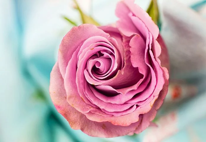
Here, the petals do not extend straight out from the center as in the previous two images. Some of them look like they curl about the center – this is definitely a characteristic that would be nice to capture in the parametrics.
Wrapping a wave around a circle
Enough waiting – it’s time to get to the actual math. How can we imitate the radially-extending petals of real-life flowers? One way is to “wrap” a wavy function graph around a circle so its waves oscillate orthogonally to the tangent line of the circle at any given angle. We can accomplish this with parametric functions.
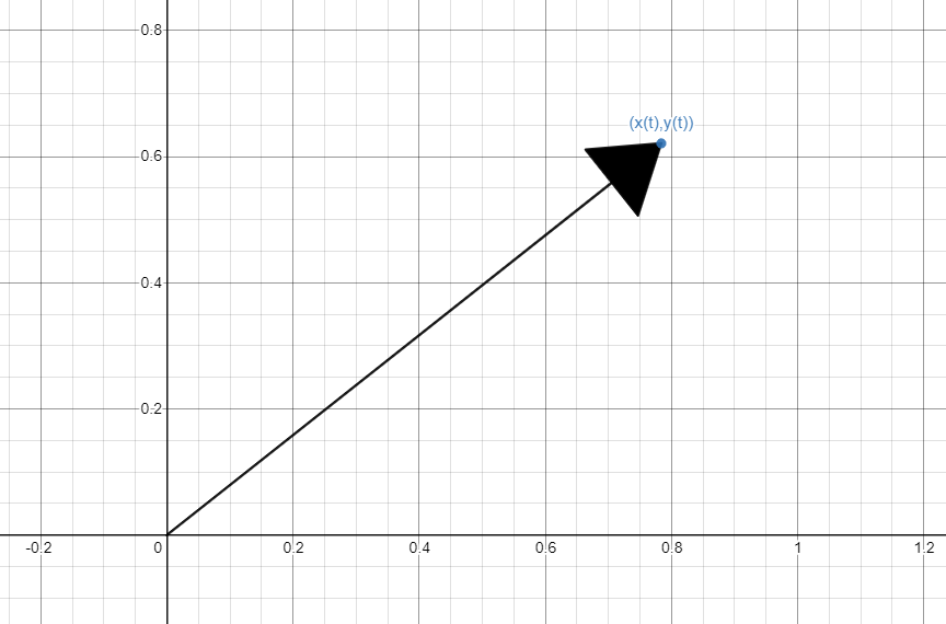
Parametric functions in the $xy$ plane map every value of a variable $t$ (called the “parameter”) on a given range to a 2-dimensional vector, or a point in space. The parametric function $f$ can be written as $f\left(x,y\right)=\left(x\left(t\right),y\left(t\right)\right)$ where $x\left(t\right)$ and $y\left(t\right)$ are functions of the parameter $t$. We can represent a vector in the plane as an arrow between the origin and the $\left(x,y\right)$ position:
To multiply a vector by a number $a$, we multiply both coordinates by $a$. By the Pythagorean theorem, this is equivalent to scaling the length of the vector by $a$ (for this reason, $a$ is called a “scalar”). For example, here’s what happens if we scale this vector by $a$, where $a$ ranges from $0$ to $1$:
vector scaling
When $a=2$, this is equivalent to placing two identical copies of the original vector tip-to-tail:
vector scale with original vector
Finally, we can make a circle. The parametric function $\left(\cos\left(t\right),\sin\left(t\right)\right)$ makes a circle when $t$ ranges from $0$ to $2\pi$. In fact, this is sometimes how the $\cos$ and $\sin$ functions are defined: as the $x$ and $y$ coordinates of a unit circle at a given angle, respectively.
circle as a parametric
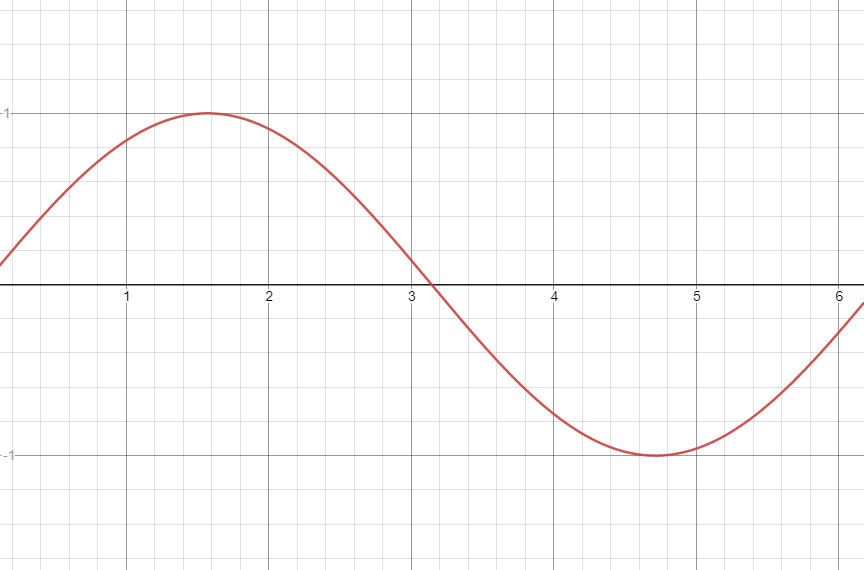
Now, we need to pick a wavy function to wrap around the circle. To begin with, let’s take $f\left(x\right)=\sin\left(x\right)$. This function has a couple important properties for our purposes. It’s periodic, meaning it repeats itself at regular intervals. Even better, the period of $\sin\left(x\right)$ is equal to the $t$ range of the circle. It repeats itself starting at every integer multiple of $2\pi$. It also has a smooth, natural-looking wave shape:
How can we wrap this around the circle? Every value of $\sin\left(x\right)$ is a scalar, so we can multiply it by a vector. If we multiply $\sin\left(t\right)$ by the circle vector $\left(\cos\left(t\right),\sin\left(t\right)\right)$ at every value $0\leq t\leq 2\pi$, we get a circle scaled by the corresponding $\sin$ value at each angle $t$. This gives the equation:
$$\sin\left(t\right)\cdot \left(\cos\left(t\right),\sin\left(t\right)\right)$$
To give some space between the petals and the origin, we can add another unscaled circle vector to this equation:
$$\sin\left(t\right)\cdot \left(\cos\left(t\right),\sin\left(t\right)\right) + \left(\cos\left(t\right),\sin\left(t\right)\right) $$
$$=\left(1+\sin\left(t\right)\right)\cdot \left(\cos\left(t\right),\sin\left(t\right)\right)$$
In the following animation, the red arrow shows how the addition of the $\sin$-scaled vectors changes the curve.
cardioid
That shape is called a cardioid. It’s a well-known shape that arises in many contexts all over math. But wait – that doesn’t look anything like a flower. Let’s introduce an integer constant $b$. If we plot $\sin\left(bx\right)$ where $b=1,2,3,4$, we get this:
wave frequency
It multiplies the frequency of the wave by $b$. For example, if $b=3$, the wave will go through $3$ full periods on $0\leq x \leq 2\pi$ instead of just one. Using the same method as before, we can wrap this higher-frequency wave around a circle. Here’s the resulting equation:
$$\left(1+\sin\left(bt\right)\right)\cdot \left(\cos\left(t\right),\sin\left(t\right)\right)$$
When plotted, it gives better results. If $b=2$:
two petals
If $b=3$:
three petals
If $b=4$:
four petals
And so on. The value of $b$ equals the number of petals that the flower has. In other words, you could call the cardioid a “one-petal flower”!
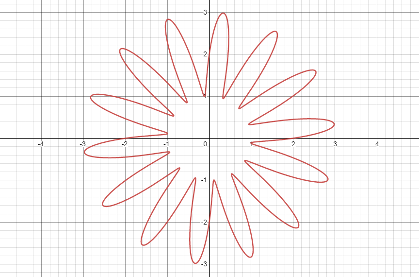
If you add other circle to the parametric to push it further away from the origin and let $b=14$, you end up with a shape close to the first reference image:
Other wave shapes
As long as the wavy function that we wrap around the circle has a period length that is evenly divides into $2\pi$, the resulting parametric will start and end in the same place to create a closed flower. It doesn’t need to be $\sin\left(x\right)$. We can define the “general single-layer flower function” as
$$\operatorname{W}\left(t\right)=\left(2+f\left(bt\right)\right)\cdot\left(\cos\left(t\right),\sin\left(t\right)\right)$$
where $f$ is the wavy function. If $f(x)=\sin\left(x\right)$, we get the above flower shapes.
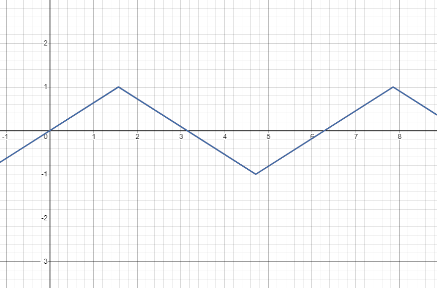
What if we want the petals to be pointier? We could imagine a function with the same overall shape as $\sin$, but with more jagged peaks and troughs. There are many ways to obtain such a function. Some examples are:
$$f(x)=\frac{2\arcsin\left(\sin\left(x\right)\right)}{\pi}$$
This takes advantage of the domain restriction on $\arcsin\left(x\right)$ and the fact that $$\arcsin\left(\sin\left(x\right)\right)=x$$ to create repeating straight lines.
Alternatively,
$$f(x)=\operatorname{abs}\left(\frac{2}{\pi}\left(\operatorname{mod}\left(x-\frac{\pi}{2},2\pi\right)-\pi\right)\right)-1$$
This uses the modulo operator (“mod”) which is a fancy name for taking the remainder of the division of two numbers. Both of these have the exact same graph:
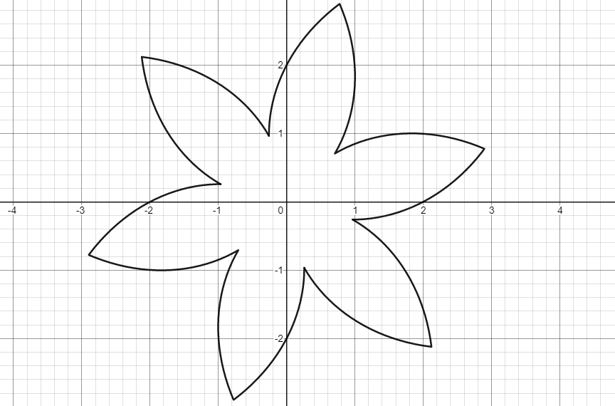
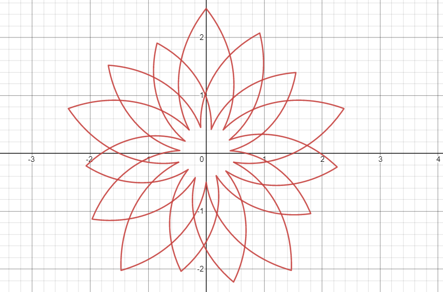
If we plug this into $\operatorname{W}\left(t\right)$ as $f\left(x\right)$, we get flowers with pointier petal ends, as expected:
Another example is
$$f\left(x\right)=\sum_{n=1}^{50}\frac{1}{2n-1}\cos\left(\left(2n-1\right)x\right)$$
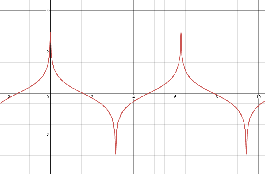
which looks very nice as a flower:
There are infinite possibilities. If you’re curious, try some different functions – believe me, it’s much more satisfying to discover these shapes on your own.
Layering petals
How can we replicate the layered look from the second reference image? Here, it will be easier to look at one solution and work backwards. The final general equation for layered flowers is
$$W_{\text{layered}}\left(t\right)=\frac{1}{1+dO\left(t\right)}\left(c+f\left(\frac{2\pi}{L}O\left(t\right)+bt\right)\right)\cdot\left(\cos\left(t\right),\sin\left(t\right)\right), \ \ 0\leq t \leq 2\pi L$$
Where $O\left(t\right)=\operatorname{floor}\left(\frac{t}{2\pi}\right)$, $L$ is the number of layers, $b$ is the number of petals per layer, $c$ controls how much space between the origin and first layer of flowers, and $d$ controls how much each layer diminishes in size. We can break this equation down into pieces to see how it works.
First, consider $O\left(t\right)$. It counts how many times the curve has traveled around the origin, or how many closed loops the curve has made. Before the curve has made a full closed loop, $t$ is less than $2\pi$ because a single layer takes an interval of length $2\pi$. So $\frac{t}{2\pi}$ is less than $1$, which $\operatorname{floor}$ rounds down to zero. Once the first loop is completed, $t$ will be between $2\pi$ and $4\pi$ so $\frac{t}{2\pi}$ is between $1$ and $2$, so $\operatorname{floor}$ will round it down to $1$. Continuing like this, $O\left(t\right)$ counts the number of completed loops.
Now we can look at the scale factor term $1/\left(1+dO\left(t\right)\right)$. This factor is multiplied by the rest of $W_{\text{layered}}$, so it scales the entire parametric. Recalling the meaning of $O\left(t\right)$, the denominator increases by $d$ every complete loop, or every complete interval of $2\pi$. A high value of $d$ would cause the denominator to increase quickly, thus rapidly decreasing the scale factor. $d=0$, on the other hand, would mean the denominator does not increase at all. Therefore, higher values of $d$ cause each layer (full loop) to be significantly smaller than the last, while smaller $d$ values cause the layers to decrease in size more slowly.
The rest of $W_{\text{layered}}$ closely resembles $W$. The main difference is the argument to the wavy function $f$. We’ve added the term $\frac{2\pi}{L}O\left(t\right)$. This once again involves $O\left(t\right)$, so it is immediately clear that it depends on the count of full loops. More specifically, $\frac{2\pi}{L}$ is added to the argument of $f$ each full loop. Where did that number come from? Before answering that, let’s take a look at what adding a constant to the argument of a periodic function does in general. Take the function $\sin\left(t\right)$ as an example. If we add a constant $k$ to the argument (making the function $\sin\left(kx\right)$), here’s what it looks like:
translation
The function shifts to the left by $k$ units, but notice how the line connecting $\left(0,\sin\left(k\right)\right)$ and $\left(2\pi, \sin\left(2\pi+k\right)\right)$ is always horizontal. This is a consequence of the periodicity of the function: values of the function at inputs that are $2\pi$ apart are always equal. If we then wrap this around the a circle like before, the endpoints will remain connected because they are still scaled by the same value. The petals are rotated counterclockwise about the center as $k$ changes because the function being wrapped in a circle is shifting to the left. Rotating is really just shifting around a circle. Since any function that repeats itself an integer number of times on an interval of length $2\pi$ is also periodic every $2\pi$, shifting it by $2\pi$ will always leave it looking exactly the same. This is where the $\frac{2\pi}{L}$ comes from. The shift amount from layer to layer is $\frac{1}{L}$ times the amount of rotation that would leave a layer looking unchanged. This makes sure each layer is evenly spaced between the next and last layers, as noted in the second flower reference image.
That’s it! Example layered flower: let $f\left(x\right)=\frac{2\arcsin\left(\sin\left(x\right)\right)}{\pi}$ (the pointed petal function from above), $d=0.1$, $c=1.5$, $L=3$, and $b=5$. Here’s what it looks like:
Follow link to experiment with graph: https://www.desmos.com/calculator/fi7anttzqi
Non-radial petals
So far, all the designs involve petals that extend radially out from a circle centered at the origin. You could draw a ray starting at the origin at any angle and it would cross the parametric exactly once (per layer). As noted above, some real-life flowers do not have this property. What if we want to model flowers with petals that curve around the center circle? This more intricate design comes at the cost of greater complexity, but we can still do it.
Wrapping some $y=f\left(x\right)$ around a circle no longer suffices because we may need more than one point at a given angle. Functions of $x$ always pass the “vertical line test”, meaning each value of $x$ never maps to more than one $y$. Instead, we are going to wrap another parametric function around the circle in a looser sense of the word “wrap”. At every angle around the circle, we move some amount of units in the direction of the tangent vector, and some amount of units in the direction of the orthogonal vector. Any point in the $xy$ plane can be represented as the scaled sum of the standard basis vectors $\hat{\imath}=\left(1,0\right)$ and $\hat{\jmath}=\left(0,1\right)$. For example, the point $\left(4,2\right)$ is equal to $4\hat{\imath}+2\hat{\jmath}$:

These basis vectors are arbitrary, however. We can define our own basis as the unit (length 1) tangent and orthogonal vectors to a circle at a given angle. A point can then be converted to this basis so its coordinates are relative to the point on the circle at that angle. This process is repeated at every angle from $0$ to $2\pi$ so we can define a point on the parametric curve. How do we get the unit tangent and unit orthogonal vectors to a circle at a point? There are several ways, but the most straightforward method involves differential calculus. If you don’t know calculus, it’s fine to treat this part as a black box that gives the desired vectors.
Recall that the standard parameterization of a circle is $\left(\cos\left(t\right),\sin\left(t\right)\right)$. The tangent vector $T\left(t\right)$ is equal to the derivative of this parametric function with respect to $t$:
$$T\left(t\right)=\frac{d}{dt}\left(\sin\left(t\right),\cos\left(t\right)\right)=\left(-\sin\left(t\right),\cos\left(t\right)\right)$$
Each vector generated by the circle parameterization has length $1$ by the pythagorean identity $\sin^2\left(t\right)+\cos^2\left(t\right)=1$, so this is already the unit tangent vector and there is no need to divide by the magnitude. The vector $\left(-y,x\right)$ is perpendicular to $\left(x,y\right)$ by reflection. Therefore, the outward-pointing unit normal vector $P\left(t\right)$ is
$$P\left(t\right)=\left(\cos\left(t\right),\sin\left(t\right)\right)$$
because the tangent and normal vectors are orthogonal. This is unit length because reflecting a vector does not change its magnitude. Here’s what the vectors look like at all angles:
circle vectors
We can convert a parametric to this alternative basis by multiplying its $x$ coordinate by the tangent vector and $y$ coordinate by the orthogonal vector. In other words, for the periodic petal function $f\left(t\right)=\left(f_{1}\left(t\right),f_{2}\left(t\right)\right)$, the equation
$$wT\left(t\right)\cdot f_{1}\left(bt\right)+wP\left(t\right)\cdot f_{2}\left(bt\right)$$
gives $f$ converted to the new basis where $w$ is an arbitrary scale factor and $b$ has the same meaning as always. We can then add on the usual $c\cdot\left(\cos\left(t\right),\sin\left(t\right)\right)$ to push the parametric away from the origin. The resulting general equation is
$$W_{\text{parametric}}\left(t\right)=wT\left(t\right)\cdot f_{1}\left(bt\right)+wP\left(t\right)\cdot f_{2}\left(bt\right)+c\cdot\left(\cos\left(t\right),\sin\left(t\right)\right)$$
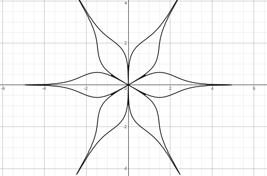
Now, to create the petals. The petal shape really can be anything you want. A good-looking example is $f_{1}\left(t\right)=2\left(\cos\left(\frac{t}{2}\right)\sin\left(\frac{t}{2}\right)\right)^{2}-1$ and $f_{2}\left(t\right)=\sin\left(t\right)$. Here’s what that looks like on $0\leq t \leq 2\pi$:
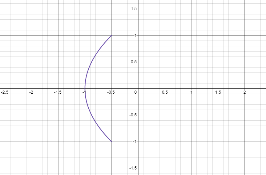
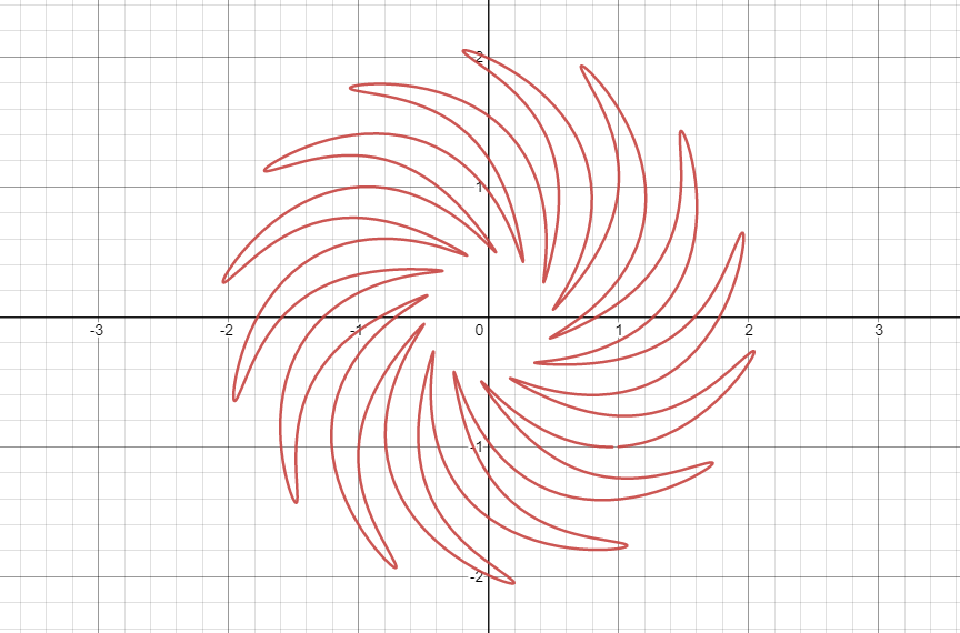
This parametric is periodic, so it retraces itself over at intervals of $2\pi$. When plugged into $W_{\text{parametric}}$ with $b=14$, $c=1$, and $w=1$, it looks like this:
And here, you can see it being swept out by the vectors ($b$ reduced to $6$ for clarity):
sweeping out path
Follow link to experiment with graph: https://www.desmos.com/calculator/kuopa7axoc
Moving to three dimensions
No matter what the subject, there will never be a post on this site without 3D surfaces wedged in somehow. We can use similar equations to generate parametric flowers in three dimensions. In 3D, there is even more artistic customizability. The derivation of these equations goes beyond the scope of this post, which is already quite long. Anyway, here are some example equations:
$$X\left(u,v\right)=\left(\frac{v}{1+0.25\operatorname{floor}\left(\frac{u}{2\pi}\right)}\right)\left(1+\sin\left(5u+\pi\operatorname{floor}\left(\frac{u}{2\pi}\right)\right)\right)\cos\left(u\right)$$
$$Y\left(u,v\right)=\left(\frac{v}{1+0.25\operatorname{floor}\left(\frac{u}{2\pi}\right)}\right)\left(1+\sin\left(5u+\pi\operatorname{floor}\left(\frac{u}{2\pi}\right)\right)\right)\sin\left(u\right)$$
$$Z\left(u,v\right)=\left(\cos\left(u\right)-X\left(u,v\right)\right)^{2}+\left(\sin\left(u\right)-Y\left(u,v\right)\right)^{2}+\sqrt{X\left(u,v\right)^{2}+Y\left(u,v\right)^{2}}+\frac{1}{4}\operatorname{floor}\left(\frac{u}{2\pi}\right)-2$$
When plotted on $0\leq u \leq 12\pi$ and $0 \leq v \leq 1$, it looks like this:


Thanks for reading!
This post was submitted to the SoME1 contest.