As is tradition, I’ll share a few of my favorite recent Desmos graphs. Since last year, Desmos has done some significant updates, including performance improvements and new feature implementations. The largest new features are polygon lists, actions, and list comprehensions, which essentially trivialize many things that were previously difficult on Desmos. While this is obviously great for Desmos (and the calculator is much better as a result), it takes away a lot of the challenge. Creating an impressive Desmos graph used to take more skill and effort than it does now. So I’ll include graphs using the new features, but note that some of the more simplistic looking graphs are actually the ones that took the most effort. I’ve made 200+ graphs since the last post. This post is skewed towards the most recent.
3D Graphing

To get it out of the way : here are all the 3D plotting graphs. These all mimic features of MathGraph3D. The image above shows a 3D surface with occlusion and normal vector-based coloring created BEFORE the polygon and list comprehension update. It runs very slowly (loads in about 25 seconds) because the entire surface is rendered as a single parametric equation. This was my chef d’oeuvre at the time, but the same thing can now be done easily in real time using polygon lists.
Original 3D Plotter (before update – warning : long load time) : https://www.desmos.com/calculator/lwdugtwnem
Real time 3D Plotter : https://www.desmos.com/calculator/3o8pkr1tza
Surface of Revolution Plotter : https://www.desmos.com/calculator/ft1ydzq2an
Parametric Surface Plotter : https://www.desmos.com/calculator/nyizgwkaj0
Cylindrical Coordinates Plotter : https://www.desmos.com/calculator/qekdilsvdv
Space transformation
This represents a function $f : \mathbb{R}^2 \to \mathbb{R}^2$. It takes every point in a grid in the plane and linearly interpolates it to its output when passed into $f$. The animation is not really inherent to the function, but it’s a nice way of visualizing how the inputs get mapped to their outputs.
Link : https://www.desmos.com/calculator/g3cxl3tynv
3D Version : https://www.desmos.com/calculator/xgwoiwgicc
University of Pittsburgh Logo
The crest of the University of Pittsburgh, my university, because why not.
Link : https://www.desmos.com/calculator/cxvgs8mfog
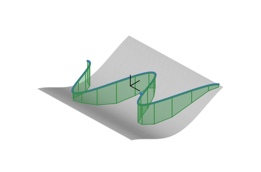
Bézier Surfaces

You’ve probably heard of Bézier curves or Bézier splines, but have you heard of Bézier surfaces? A Bézier surface is basically the 3D generalization of the Bézier curve. You can click the shuffle button in the graph to regenerate the anchor points to get a new random surface.
Link : https://www.desmos.com/calculator/ppugugydtg
Maximal Ascent
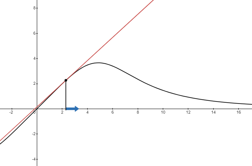
If not for parametric flower design, this would have been my SoME1 topic. The gradient points in the direction of steepest ascent, and the reason why is very intuitive if you are able to visualize it properly. Taking the partial derivative with respect to a certain variable given fixed values for the other variables is equivalent to taking the 1-dimensional (single variable) derivative at that cross section. This graph shows how the single variable derivative always points in the direction of steepest ascent. The gradient is the vector of all these cross-sectional derivatives as components, thus why it points towards the direction in which the function increases the quickest.
Link : https://www.desmos.com/calculator/0fgonhzjmd
Perceptron with Gradient Descent
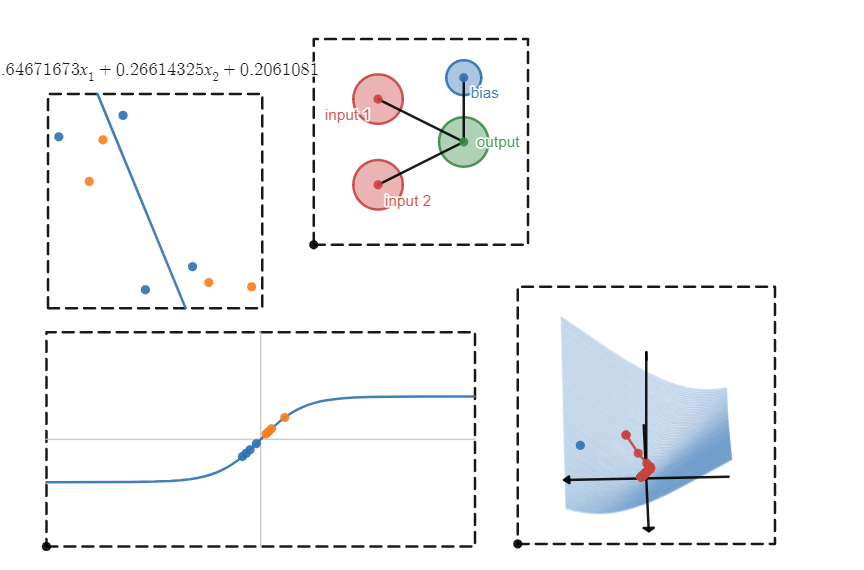
This is a working machine learning model in Desmos. It simulates a single perceptron, the simplest of machine learning models. I created this as a visual aid for a presentation I gave to the math club at my university about perceptrons, log loss, and gradient descent. The perceptron performs a linear classification task. If the orange and blue points are positioned by the user to be linearly separable, the model will correctly learn the decision boundary. The top left panel shows the input data and decision boundary, the top right shows the model schema, the bottom left shows the model’s predictions, and the bottom right shows the log loss error as the gradient descent algorithm runs.
Link : https://www.desmos.com/calculator/h0ichtaivm
Path Follower
This is based on Daniel Shiffman’s path following procedure, which comes from part of a series of simulating natural movement. Shiffman’s code works for following paths defined by straight lines. The vehicle in the graph follows any parametric defined path according to the same algorithm. The biggest challenge with this graph is computing the closest point to the vehicle at any given time. It’s not really analytically solvable, so it has to be done numerically. I had two options in mind for this : Newton’s method and gradient descent. Although I prefer Newton’s method, I ended up going with a hybrid of the two for performance reasons. It uses a high-precision estimation to find the first closest point, then uses the previous closest point as the initial guess for the next computation so fewer iterations are required.
Link : https://www.desmos.com/calculator/fzotpw8hgh
Scalar line integral
This visualizes a Riemann sum for the line integral over the scalar field defined by $f(x,y)$ and represented by the grey surface. It’s an imitation of the MathGraph3D feature that does something similar.
Link : https://www.desmos.com/calculator/mqia67wnd2
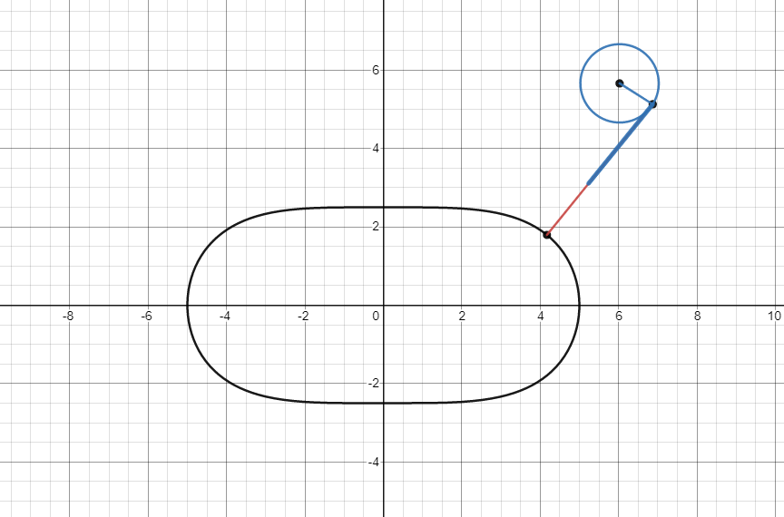
Generalized “Hypotochroid”
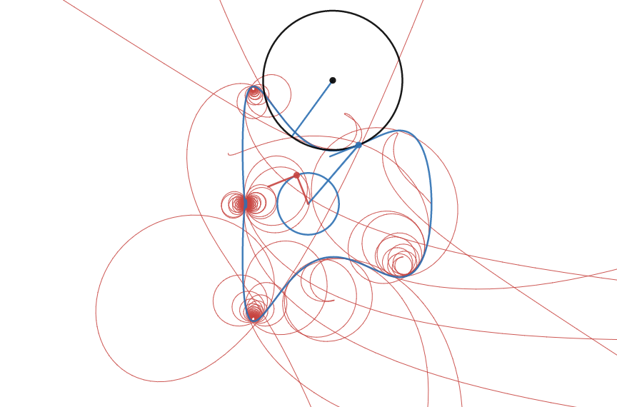
A hypotrochoid is a type of curved traced out by a circle rolling around another circle. I generalized this notion to a circle rolling around an arbitrary parametric. The trouble is, unlike a circle, an arbitrary parametric does not have constant curvature. So I resize the rolling circle to half the radius of curvature at the point of intersection. It rolls without sliding such that the arc length rolled on the path is equal to the arc length rolled by the circle.
Link : https://www.desmos.com/calculator/v8c0lvnlsk
Car with Square Wheels

This shows a car driving smoothly on a track composed of catenaries. It would be as easy to drive this car as it is to drive a car with round wheels on a flat track. The car does not move up and down because the sum of the track height and the distance from the wheel center to the bottom of the wheel is constant. The existence of such a track is non-obvious, but you can do it for any regular polygon (and other shapes, too).
Link : https://www.desmos.com/calculator/qt29nvqdck
Thanks for reading! As I said, I have far too many graphs to include in this post, so I’m going to cap it here at 10.