Finally, after a few months of promising this post, here it is. This series focuses on the creation of the original version of my 3D plotting software MathGraph3D. The first part was about the overall structure of the software. This second part is concerned with all algorithms for smoothing and optimizing surfaces.

The basic idea of writing a program to plot 3D surfaces isn’t too difficult once you get all the 3D space handling techniques covered. A naive script would map a mesh of input points (in the case of a function, samples from the xy plane) to a value, triangulate it in some way, and draw the resulting polygons. This would work pretty well in most cases. However, math is a messy universe; not all functions and surfaces are simple, smooth, continuous, or generally well-behaved. Even when they are, they’re not necessarily readily compatible with being programmed into a computer.

The goal of an advanced algorithm is to approximate a mathematical surface with the minimum number of sample points possible while capturing the maximum amount of detail. Surface generation is a constant battle between performance and accuracy. The higher the accuracy, the more polygons the graphics library is required to render. High performance means fewer points which means less detail. A certain amount of this tradeoff can be handled by preprocessing and storing informaiton in memory. Obviously, this leads to higher detail and performance at the expense of more memory usage. Here are some of the specific problems that an advanced surface generation algorithm addresses:

• Clipping – for some reason, I talked about this in the first post
• Optimal sample point distribution.
• Discontinuity handling where the function is undefined on a portion of the input space.
• Jump or pole discontinuties.
• Polygon splitting
• Consistent polygon vertex orientation

Now, I’ll explain each of these problems and their corresponding solutions in greater detail (as implemented in python MathGraph3D).

Optimal Sample Point Distribution

This is the hardest surface generation problem to solve. Surfaces of mathematical functions will be more detail-heavy in certain areas than others. I will present several algorithms here. Which one of them works the best is a matter of circumstance. Most of them can be used simultaneously.

• Reducing the sample space to the smallest axis-aligned bounding boxes containing no undefined inputs and redistributing the unused points elsewhere.

This is quite easy to do. In the preprocessing phase, generate a dense grid of sample points and test if the function is defined on them. Find the points with the most extreme values in each input direction (x and y). Then, reduce the input space to the box with edges containing these points.

• Adaptively dividing the surface based on some error metric.

This method can be used when a user wants to be sure that the error in surface detail is no greater than a specified amount. Compute some error metric $E$ for all points in the input space. Where $E$ is high, divide the polygon into 2 or 4 parts by slicing it down the middle. This is repeated until the sum error between the polygon approximation and the actual surface is below a specified threshold.

• Distributing points in the input plane according to highest sum of second derivatives.

Again, precompute a dense sample grid. Ensure there are enough points for the edges of the input region. Then, disperse the points among a number of subdivisions of the input region according to the average of the sum of the magnitudes of the second derivatives at each point in the subdivision. Then, disperse the points evenly in each subdivision.

• Distributing so that every polygon in the surface approximation has equal surface area.

General methods exist for computing a parameterization of a surface such that changes in the input parameters yield equal changes in the surface area of the output. This is overkill for the purpose of surface generation, and it’s not even exactly what we’re after. We want all the polygons to be equal-area, not regions of the actual surface. Once again, a dense grid is generated. Then, each polygon starts at zero surface area and is expanded just until its surface area exceeds the average. It is slightly reduced with linear interpolation so it is then very close to exactly equal surface area (assuming sufficiently high density).

This might be hard to visualize, so consider the 2D equivalent: equal arc length points on a 1D curve. To obtain such points, you can generate a dense sample. Starting on the left and moving right, you choose the line endpoints one at a time. Start with a segment of length zero, and expand the right endpoint by making it the next in the sample space until the length of the segment is just over the desired arc length. Then, backtrack to some point between the endpoint and the previous sample point by linear interpolation.

The method of equal surface area performs suprisingly poorly in some cases. Most of the time it works well, but it is probably the least reliable algorithm in this list.

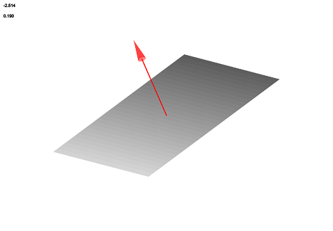
• Detecting “directionally simple” regions.

“Directionally simple” is not an official, accepted, or known term, thus the quotes. If a region of a surface is directionally simple, it can be replaced by merely two sample points in some direction without any loss of detail (i.e. it is linear in one direction). Replacing directionally simple regions can greatly reduce polygon count in certain contexts. For example, it reduces all planes down to a single polygon.

It’s best practice to allow for some small numerical deviation from a plane. With sufficiently small deviation, the human eye will not be able to tell the difference even if it is not quite exact. This expands the category of functions that can be represented with a much lower polygon count (such as the exponential bell surface). If applicable, the removed superfluous sample points may be redistributed elsewhere.

• Edge contraction with an error metric based on treating polygons containing each point as planes and computing deviation from the ideal surface (this is essentially a generalized RDP line simplification algorithm)

Like adaptive division, this method ensures that there is no more than a specified maximum error between the polygon approximation and actual surface. The error at a point $P$ is defined to be the sum of the distances between the planes formed by the adjacent polygons and the surface. If the error is less than the specified amount, the algorithm performs edge contraction. Edge contraction is when one of the edges in a polygon is contracted to a single one of its endpoints and the resulting degenerate polygon is removed.

To visualize this algorithm, consider the 2D equivalent (where the error metric is the distance between the segment and the curve). The following picture shows the finite approximation using equally spaced sample points in red. The reference curve is in blue.

And the next picture shows the finite approximation after the algorithm has been run. Note that the same number of points are used in both approximations. The black dots at the top show the placement of sample points. The second approximation is obviously much better and preserves the structure of the curve.

This method is very effective and feature-preserving. However, it requires a surface triangulation, which is not how MathGraph3D operates. So, once the algorithm is run on a triangulated surface, the triangles are converted to polygons with more sides at the end.

Undefined Surface Discontinuity

Functions can be undefined on oddly or irregularly shaped regions in the input plane. For example, the top half of a sphere is only defined on a circle in the plane. With a naive algorithm that samples points in a regular rectangular grid, this results in something like this:

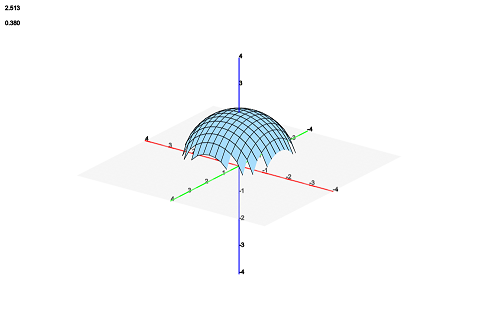
This is very ugly and obviously not representative of the mathematical half-sphere. After adjusting the position of sample points, the surface looks like this:

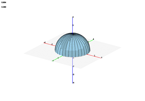
Clearly, this is much better. Though this takes advantage of the unused point redistribution as described above, that is insufficient to produce the pictured smooth half-sphere. So, we must also do some readjustment on the border of the defined region of the function.

Continuing with the example of a half-sphere, consider the region in the xy plane on which the function is defined, as shown by the interior of the black circle in the following picture. The picture also shows a regular rectangular grid of sample points in blue.

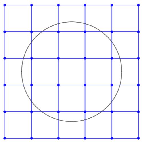
Per the algorithm above, all the points that are outside the smallest bounding box of the circle will be redistributed to increase the sample density on the area of definition. Notice, however, that none of the blue points hit the edge of the circle. To resolve this problem, look at all the pairs of points such that the edge between them intersects the circle.

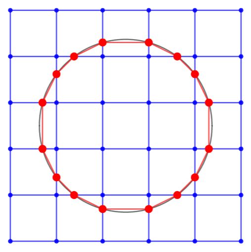
Notice how closely the red intersection points approximate the perfect circle of definition, even with such a low density (6×6). So, how can these points be found? Again, we resort to frontloading the processing of the surface so it doesn’t have to be computed every frame. Take the pair of points on each intersecting edge. Using a search with an arbitrary number of iterations, locate the x or y value that is on the boundary of definition. For a given point, if the surface is defined, move closer to the internal point on the edge. Otherwise, move closer to the external point on the edge. The distance by which we “move closer” decreases each step.

Jump and Pole Surface Discontinuity

Everybody reading this is probably familiar with infinite and removable discontinuities in two dimensions. The same types of things exist in three dimensions, and they pose problems for surface generation. Consider the example of the complex function $f\left(z\right)=\sqrt{z}$. With a naive surface generation algorithm, this is the result of plotting $\left(x,y\right)\to \text{Im}\left(f\left(z\right)\right)$:

That row of tall polygons is not supposed to be there. This is a good example of what happens with a basic algorithm. The sample interval skips over the discontinuity, completely unaware that it shouldn’t be connecting those two portions of the surface with a polygon. The original version of MathGraph3D contained no perfect solution to this problem. As a matter of fact, no version of MathGraph3D has a solution to this that works 100% of the time. It turns out that identifying this type of discontinuity is quite difficult because most of its defining characteristics can be closely mimicked by valid, continuous functions. With that being said, it is possible to resolve the problem in many cases without issue.

In each input direction (at the regular step length, not a denser one), compute the first derivative. If there is a large, sudden spike in the derivative along with a derivative sign change, assume that it is a jump and remove the polygon. In the example, the result looks like this:

Personally, I’m not a fan of this algorithm. It’s cheap and hacky. Yet this remains in use in MathGraph3D to this day because I can’t think of a better one.

Polygon Splitting

There are two reasons to split a polygon. First, if it is intersecting with another polygon. Second, if it is so long or tall in one direction that it cannot be consistently sorted correctly relative to the other polygons.

In the first case, the polygon must be split because otherwise it is impossible to correctly sort the polygons so the correct portions of the are occluded (not visible). For this reason, it suffices to split just one of the polygons and leave the other one untouched.

Splitting a polygon along an intersection line with another is a simple matter of computing the line of intersection between two planes, which is a basic algebra computation. The difficult part of this algorithm is determining whether two given polygons overlap. The standard surface resolution for MathGraph3D is 32 by 32, for a total of 1024 polygons. If there are two surfaces, this means there are 1024 * 1024 = 1,048,576 intersections that need to be checked, which is not feasible. This can be worked around by dividing 3D space into an octree. Basically, polygons are only tested for intersections with the other polygons in a local area. As it can be expensive to test for intersection for 3D polygons, the algorithm first checks if the shadows of the polygons when projected onto the xy plane overlap to quickly rule out intersections. Obviously, if the shadows don’t overlap, the actual polygons don’t either.

In the second case, the polygon must be split because once again this situation makes it impossible to sort the polygons in all orientations. Resolving this case is trivial. Just split the polygon at its center to create two new polygons.

Consistent Polygon Orientation

In order to make sure the vertices of a polygon are drawn in the correct order, they must be sorted in a consistent direction (clockwise or counterclockwise about the center from the same reference point). This also establishes a consistent normal vector for each polygon so that the normal vector and inverse normal vector color styles work.

First compute the barycenter (center of gravity) $C=\left(c_1, c_2, c_3\right)$ of the polygon. Then, sort each vertex $A=\left( x,y,z \right)$ by the following function:

$$f(A)=\text{atan2}\left( y-c_2, x-c_1 \right)$$