This series focuses on the creation of the original version of my 3D plotting software MathGraph3D. The first part was about the overall structure of the software. The second part was concerned with all algorithms for smoothing and optimizing surfaces. This third part discusses coloring, lighting, and styling the objects that MathGraph3D plots. I’ll try to keep this part shorter than the other ones… posts in this series have a tendency to spiral out of control.
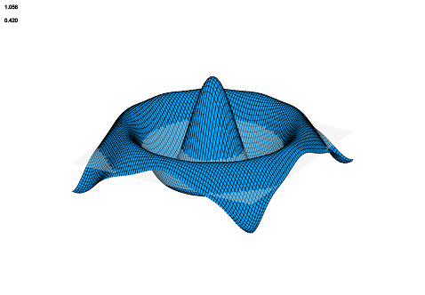
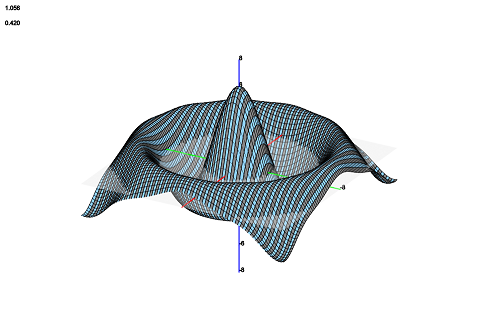
In MathGraph3D, every plottable object has an attribute of type ColorStyle that stores information about how the surface or curve should be styled. All ColorStyle objects contain a method next_color() which takes in the properties of a polygon and return its proper color. There are two types of coloring in MathGraph3D: static and dynamic. Static coloring is only done once at the time of surface generation. This means that the color of the polygons in the surface never change. The second type, dynamic coloring, is recomputed every time the plot updates. Dynamic coloring is used for lighting purposes only; the rest of the coloring types use static coloring. All coloring types allow transparency and the option to draw a grid mesh on the surface.
Solid Color
This one is pretty self-explanatory. The solid color ColorStyle returns the same color, as specified by the user, regardless of the properties of the polygon it is passed.
Checkerboard Pattern
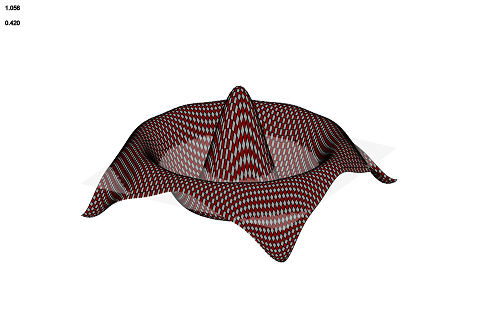
The checkerboard ColorStyle returns alternating rows of alternating columns of two different colors as specified by the user. The next_color method receives the index i that represents the polygon’s row in the surface and the index j that represents its column. To achieve the desired effect, the method returns one color when mod(i+j, 2) is equal to zero and the other color when it is equal to one.
Linear Gradient
The gradient ColorStyle takes the number of total polygons in the surface and linearly maps all polygons in order between two colors. The algorithm is as follows. Compute the proportion $p = \left(\text{Current polygon index}\right) / \left(\text{Number of polygons}\right)$ Let $c$ (for “complement”) be $1-p$. Then the color $100p$% from color 1 to color 2 is $c \cdot \left(\text{color 1}\right) + p \cdot \left(\text{color 2}\right)$.
Checkered gradient

This essentially combines the previous two styles. It does a gradient style, but at checkerboard intervals, it darkens the color by 20%.
Vertical stripes

The vertical stripes ColorStyle returns one color when the column index is even, and the other when it is odd. This results in stripes of color parallel to the y-axis.
Horizontal Stripes
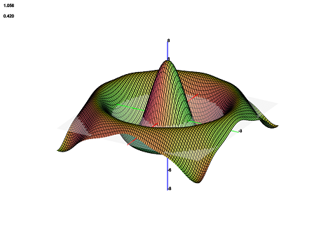
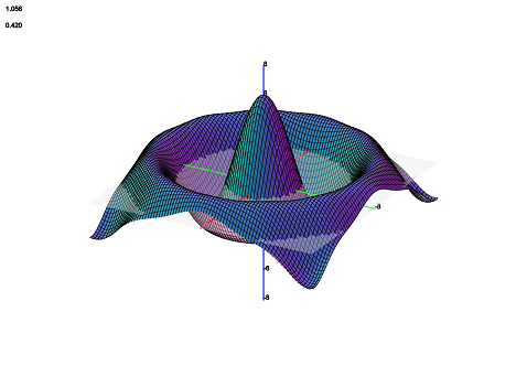
Horizontal (parallel to the x-axis) stripes are made by repeating the vertical stripe procedure but with the row index. For functions (such as the one shown), it doesn’t make any sense to distinguish between vertical and horizontal stripes due to rotational symmetry about the z-axis. However, for other types of surfaces that may have more than one point associated with each (x,y) pair, it is more useful.
Output intervals

The output intervals ColorStyle is like projecting a contour map onto the surface. The z value attained by the midpoint of a polygon is normalized between -1 and 1 using the minimum and maximum z values. The resulting normalized value is used as a position in a one-dimensional colormap specified by the user. When the normalized value is between the positions of individual colors in the map (as it will be the vast majority of the time), linear interpolation is used between the two colors on either side.
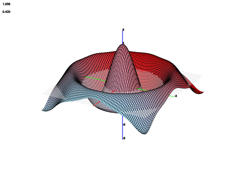
Normal vector
The normal vector ColorStyle chooses the color based on the orientation of a given polygon. This is one of the reasons that orientation of polygon vertices must be consistent, as discussed in the last post in this series. Suppose the distinct vertices $A$, $B$, and $C$ are in some polygon, in clockwise order. Then let
$$\vec{v} := \frac{A-B}{C-B} \text{ so that } \hat{v} = \frac{\vec{v}}{||\vec{v}||}$$
is the unit normal of the polygon. Compute the dot products with the canonical basis vectors for $\mathbb{R}^3$ and map the results from 0 to 255. The resulting vector gives RGB color values.
Inverse normal vector
This takes the color complement of the normal vector styling. That is, it subtracts the normal vector color from $\left(255,255,255\right)$. These last two styles are very useful because they conform to the shape of the surface.
Dynamic coloring: lighting
When lighting is used, the color must be dynamic because the shading of each polygon depends on its orientation relative to a fixed light source. Let the light source be positioned at the vector $L$ and the center of a polygon be $M$. Usually, $L$ is set to the current view direction so the light will always appear to come from the perspective of the user. Let $d_{\text{max}}$ be the maximum distance from the light source to a possible point in the current plot boundaries. Compute the 1.5 minus the square root of the distance from $L$ to $M$ divided by $0.66\sqrt{d_{\text{max}}}$. Multiply that value by the current color of the polygon and constrain each RGB value between 0 and 255 to get the color after lighting is applied.
This is a variation of flat diffuse shading. However, specular effects are simulated by the double square root (as the square root compresses large values to a greater extent than it does small values).